New Article

How to SUM by matching partial text in Excel

How to SUM by matching partial text in Excel

How to SUM by matching partial text in Excel


In this tutorial, I'm going to share another tips on
how to sum by matching partial text in Excel.


First of all, Microsoft Excel has a function called, "SUMIFS". Also has SUMIF. But I'll work here with "SUMIFS". This function allows us to sum a specific range. Based on some specific conditions. The situation of your condition is different in real life. As a result, I'm writing
how to sum by matching partial text in excel tutorial.


How to sum by matching partial text example: 

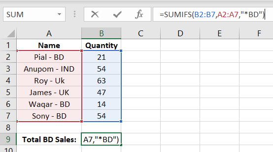
if you want to SUM only the BD based name shown in the list below, what will you do? 

How to SUM by matching partial text in Excel

Image 1: How to SUM by matching partial text in Excel


Well, in this case You can do by following below steps:

So, as you can see, I have to check all cells and find if the string “BD” appears in the cell or not, and if it does, I need to include the value in the adjacent cell in column B while doing the sum.


How to SUM by matching partial text in Excel
The above example is a case of a partial match, where I need to sum cells based on the partial match.


I'm going to use a criteria "*BD". This criteria states that, all words that ends with BD. So, i'm sure below formula (very easy for all). The formula with partial match to find the total sales quantity is:


How to SUM by matching partial text in Excel


Here is the formula:

=SUMIFS(B2:B7,A2:A7,"*BD")


The formula details are:

  • B2:B7 – This is the range, which has the values that we want to sum.
  • A2:A7 – This is the criteria range, that contains names.
  • “*BD” – I have used “*BD”. This means, any cell that ends with the string "BD" will satisfy the criteria.

Finally 21 + 14 + 54 in addition the result will show: 89


How to SUM by matching partial text in Excel article is relates to:

  • excel match function
  • excel match
  • excel match two columns
  • excel match formula
  • excel match two columns and output third
  • excel match multiple criteria
  • excel match index
  • excel match function two columns
  • excel match type
  • excel match and index function
  • excel match values in two columns
  • excel match multiple columns
  • excel match text
  • excel match columns

Comments

Popular posts from this blog

How to display an image in worksheet based on a List or based on IF condition?

Excel can show image on worksheet based on a specific IF condition. So, how to do it? Simple follow the below steps: Step by Step: Step 1: Insert images in your Excel Worksheet. Here I've inserted 5 different types of balls, Football, Cricket, Pool, Basketball, Tennis ball. Note that, All balls are placed into different cell. These are placed in Picture sheet. Image 1: 5 balls placed in 5 different cells and covered photo's wide and height Step 2: In the report sheet, design the report as you wish. I've designed in my way like below: Image 2: Kids asking to Donald Duck, which ball need to throw now Step 3: Make a drop down list "Games" in E6 cell in Report sheet from Data Validation. which is as below: Football Cricket Pool Basketball Tennis You can do an IF function here in E6 in Report sheet, which will meet a certain condition and returned Football, Cricket, Pool, Basketball or Tennis. Step 4: Now the tricky part is...

Cumulative Closing Balance like a Bank Statement in PivotTable

A Bank Employee in many case needs to calculate the Closing Balance after each transaction in PivotTable like a Bank Statement . But with the help of Calculated Field of a PivotTable , you can only calculate Field with Field . It's not possible to use a formula in Calculated Field where you can mention a single cell with Relative Reference Cell . Because a PivotTable acts like a Table format where you can work with Field or Column Name . A Helping Column (A regular column, that helps to get a partial result where formula applied) can be a good idea. But there is an option in PivotTable by which you can Calculate Cumulative . In this article I will show you, how you can do it. Calculating with Formula: Assume that, you have an Excel file with Debit and Credit transaction of an Account . Image 1: Sample Bank Statement In a Bank Statement , Month wise Cumulative Balance is important. In the Excel sheet, as above, it is very easy to use a formula and calc...

Value Paste and Formula Paste

In many case, in our professional life, we need to do Copy and Value Paste or Copy and Formula Paste in all most always. Those employees, who works under MIS Department, have to do it lots of time in a single day to prepare reports. It is very time costing task in Office. Many of us use Excel Menubar to do it, others are using Keyboard Shortcut by pressing ALT key (like for Value Paste Press ALT+H+V+V and for Formula Paste Press ALT+H+V+F ). But did you noticed that, these two ways strongly need your attention to do this task. More clearly, if you choose Value Paste from Menubar , then what you need to do? First you should take the mouse in Hand Wheel the mouse in Home menu Then Click on Paste Then you pressure your eyes to find the Value Paste icon And then Click on it to paste it These all steps can take more than 1 second. Am I right? Below is an image of this process: Image 1: Value Paste from Home Menu On the other hand, if you choose the shortcut f...