This Vlookup function is also known as Vertical Lookup. It is commonly used in Excel to match a lookup value from a column, and returned value from another column where lookup value matched. The match type can be define as Exactly Match or Approximate Match (Ascending Order). It works like an English L shape as I think. This function has a lot of uses. It supports Array, so that you can customize the lookup values.
Vlookup Function:
VLookup function is a lookup function that used in Microsoft Excel for returning a specific data from a data table by matching a cell value (Number, Date, Text, etc.). More clearly, when you need to add an information of each record of a table from source table, by matching each cell value of a specific range with source data table, then you need to use VLookup function.
At present in Bangladesh, many company asks about VLookup in their Job Interview. Why? Because they feel that, if you do not have knowledge about VLookup (which is one of the most important function in Professional Life) then you can't survive in their company. And the company has no enough time to teach you on the Job. So, it is better that, you learn it and apply it in your daily life, just for practicing. I'm sure you will be a successful person in Professional Life. The structure of this function is:

=VLOOKUP(lookup_value,table_array,col_index_num,[range_lookup])
Function Details:
There are 4 arguments or parameters in this function. The first 3 argument or parameters are essential. That means if you want to use VLookup function, then you must mention the first 3 parameters. And the last parameter is optional. You can ignore it if you wish. But for a better result you need to set the 4th parameter. All of these parameters are briefed here:
lookup_value: This is the value or cell reference the VLookup will find and match.
table_array: The table array where the lookup value is present. Note that, lookup_value looks for exactly what you have given and must be in the first column of your table_array. If the lookup_value is in 2nd column and you selected table_array from 1st column, then it will returns an #N/A error.
col_index_number: If the lookup_value matched in the first column of your table_array, then which column value you wish to return need to mention here.
[range_lookup]: This is an optional parameters. If you wish to look for exact match then, use FALSE and if approximate match require then use TRUE.
Example:
Assume that, A2:C4 is a data table contains the Player, Score and Country. Write a VLookup formula in B8 cell in to find out the Country by matching Players name.
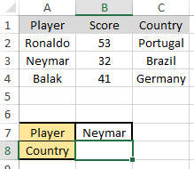
Image 1: Sample data
Solution:
Assume that, Players name already entered in a cell B7 and based on this B7 cell value the Country name will show in B8 cell.
Due to we want to return automatic result in B8, that is why we need to input formula on B8 cell. Go to B8 cell and type the below formula:
=VLOOKUP(B7,A2:C4,3,FALSE)

Image 2: Example of VLookup()
How we get the result?
B7: In Vlookup function, we have used B7 for lookup_value cell. We can use "Neymar" (with quotes) as lookup_value but it would be great if we use reference every time, and we are not typing our formula for every changed in B7 cell. So, we have used B7 as cell reference.
A2:C4: It is the data table. One point here I would like to mention that, lookup_value is in the left side of returned value Brazil. Because VLookup always returns the column number which is in right side after matched column.
3: We use this column number to return the value from third column Country based on our selected table range.
FALSE: As we want to match the value exactly what have entered, that is why FALSE has selected.

Image 3: Vlookup result returned Brazil based on Neymar lookup value
Rules:
a) Returned value Brazil must be in right side column of lookup_value Neymar.
b) Returned value Brazil must be in the first column of selected data range A2:C4.
---------------------------------------------
SUBSCRIBE our YouTube Channel
---------------------------------------------
SUBSCRIBE our YouTube Channel
---------------------------------------------