The Lookup function is used for finding a specific result from a single row or a single column, based on a lookup_value with same range of single row or single column. It does not allow 2 or more rows or columns range to find the lookup_value or returned value like others lookup function VLookup, HLookup do.
Lookup Function:
The structure of this function is:
lookup_value:
Lookup Function:
The structure of this function is:
=LOOKUP(lookup_value,lookup_vector,result_vector)
lookup_value:
The value which you want to look up in a specific row or column range.
lookup_vector:
It is a single row or single column range that contains the values to be looked up. These values must be in ascending order. That means before using this Lookup you must sort the lookup_vector range as Ascending order. Descending order will return the incorrect value.
result_vector:
It is the single row or single column range from which you want to return the value. The range size need to keep same as lookup_vector.
Example:
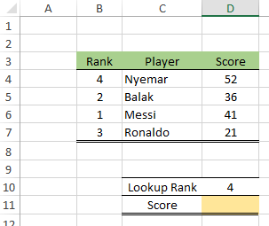
Table B4:D7 is a point table of football player. Now use a formula to find the Player Name based on their ranking.
Solution:
First the lookup_Value will search the Product column. So it is necessary to sort the Product as Ascending order. If you do not do this then it will show the wrong result.
Now in D11 cell use the formula:
Type a Rank number in the D10 cell, you will see the below result:
Note:
The Lookup function looks in a single row or single column range for a value and returns a value from the same position in a second one row or one column range.
Errors:
#N/A:
Values in the lookup_vector must be in Ascending order. If lookup_value is smaller than the smallest value in lookup_vector, it will return #N/A error.
lookup_vector:
It is a single row or single column range that contains the values to be looked up. These values must be in ascending order. That means before using this Lookup you must sort the lookup_vector range as Ascending order. Descending order will return the incorrect value.
result_vector:
It is the single row or single column range from which you want to return the value. The range size need to keep same as lookup_vector.
Example:
Table B4:D7 is a point table of football player. Now use a formula to find the Player Name based on their ranking.
Image 1: Sample data
Solution:
First the lookup_Value will search the Product column. So it is necessary to sort the Product as Ascending order. If you do not do this then it will show the wrong result.
Image 2: After A to Z sorting
Now in D11 cell use the formula:
=LOOKUP(D10,B4:B7,D4:D7)
Type a Rank number in the D10 cell, you will see the below result:
Image 3: Final result
Note:
The Lookup function looks in a single row or single column range for a value and returns a value from the same position in a second one row or one column range.
Errors:
#N/A:
Values in the lookup_vector must be in Ascending order. If lookup_value is smaller than the smallest value in lookup_vector, it will return #N/A error.


