PivotChart is a tool which is usually used for creating dashboard or viewing the report in smooth way by just changing few options in PivotTable. Basically PivotChart creates dynamic chart based on PivotTable data. Yes it is dynamic because while you changed the settings of PivotTable the data has changed and then based on this data PivotChart also changed instantly.
PivotChart added a PivotTable automatically so that, you don't need to create a PivotTable additionally.
How to create a PivotChart?
Step 1: Place the raw data in your worksheet:

Step 2: Now for creating the PivotChart based on this raw data Click the Insert menu and then Select the PivotChart from PivotChart.

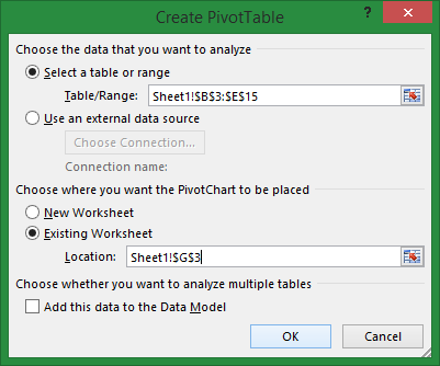
Step 3: After selecting the PivotChart, a dialog box will appear named: Create PivotChart. In this dialog box, you have to select two things. First is the data table by which the PivotChart will work and second is the location of PivotChart, where the PivotChart will pinned.

Step 4: Select the table range B3:E15 for PivotChart by Clicking the Select a table or range radio button and Click the Red upper-left directed arrow.
Step 5: With the same way, for second option Choose where you want to PivotChart to be placed, Select Existing Worksheet radio button and again select location single cell G3 by Clicking the Red upper-left directed arrow and press Enter.
After selecting these two range, Click on Ok.
Step 6: Now PivotTable and PivotChart window will display as below:

Please note that, PivotChart window is only for displaying the chart based on the Fields Settings in PivotTable window.
Step 7: Now Click on PivotTable window. Then PivotTable Fields Setting will activated with ROWS, FILTERS, COLUMNS, VALUES dragging areas. If you Click on PivotChart window then it will be FILTERS, LEGEND (SERIES), AXIS (CATEGORIES), VALUES. Both are same settings with different name. Now Drag the Title to ROWS and Sale to VALUES in PivotTable Fields setting. Then your PivotChart will looks like below:

Step 8: If you change the PivotTable field setting with more columns such as Address Field drag to COLUMNS then PivotChart will changed to below:

PivotChart added a PivotTable automatically so that, you don't need to create a PivotTable additionally.
How to create a PivotChart?
Step 1: Place the raw data in your worksheet:
Image 1: Raw data
Step 2: Now for creating the PivotChart based on this raw data Click the Insert menu and then Select the PivotChart from PivotChart.

Image 2: Select PivotChart from PivotChart
Step 3: After selecting the PivotChart, a dialog box will appear named: Create PivotChart. In this dialog box, you have to select two things. First is the data table by which the PivotChart will work and second is the location of PivotChart, where the PivotChart will pinned.
Image 3: Create PivotChart dialog box
Step 4: Select the table range B3:E15 for PivotChart by Clicking the Select a table or range radio button and Click the Red upper-left directed arrow.
Step 5: With the same way, for second option Choose where you want to PivotChart to be placed, Select Existing Worksheet radio button and again select location single cell G3 by Clicking the Red upper-left directed arrow and press Enter.
Image 4: Selecting the table location where PivotTable will appear
After selecting these two range, Click on Ok.
Step 6: Now PivotTable and PivotChart window will display as below:

Image 5: PivotTable and PivotChart window
Please note that, PivotChart window is only for displaying the chart based on the Fields Settings in PivotTable window.
Step 7: Now Click on PivotTable window. Then PivotTable Fields Setting will activated with ROWS, FILTERS, COLUMNS, VALUES dragging areas. If you Click on PivotChart window then it will be FILTERS, LEGEND (SERIES), AXIS (CATEGORIES), VALUES. Both are same settings with different name. Now Drag the Title to ROWS and Sale to VALUES in PivotTable Fields setting. Then your PivotChart will looks like below:

Image 6: PivotChart
Step 8: If you change the PivotTable field setting with more columns such as Address Field drag to COLUMNS then PivotChart will changed to below:

Image 7: PivotChart After changing Field Settings