What is Linked table?
A table which stayed in a Excel WorkSheet and connected to PowerPivot window is a Linked table. If you change any cell value in WorkSheet then it will automatically changed on PowerPivot window.
What will you need to do it?
Before importing any data through PowerPivot, you need to activate the PowerPivot window by simply clicking on PowerPivot menu and then click on Manage button under Data Model group.
After clicking on Manage button Excel will load the PowerPivot Window and it is completely separate from main Excel Window like below:
How to import data by using a linked table?
Assume that, you have the below sample data table in Sheet1 of your Excel Window:

Step 1: Select anyone cell inside the sample data. I have selected B2. Now press Ctrl+T and press Enter. This will convert the table range into a real Table Format like below:

Step 2: In Excel you may need to use more than 1 table. But the problem is, while you convert any table to a table format then it keeps the default name like Table 1, Table 2 etc.., But it is a problem to identify the specific table to calculate for further calculation. If you mention a Name for each of your table, then it would be easier to identify for calculation. In Excel you can easily create Names by pressing Ctrl+F3. Later I'll share it how to create Names. I have named the above table as SESList.
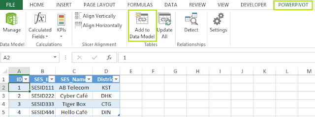
Step 3: Now click anywhere of the SESList table and then click on Add to Data Model option from PowerPivot tab.
Step 4: Finally the data will successfully imported with a new menu "Linked Table" like below image:

Please note that, SESList table name automatically assigned as table name in PowerPivot window like below image:
If you update the source data which is in Sheet1 of SESlist table from Excel Window ( not PowerPivot window), then in PowerPivot window SESList sheet will update automatically. That's the beauty of the Linked Table.
A table which stayed in a Excel WorkSheet and connected to PowerPivot window is a Linked table. If you change any cell value in WorkSheet then it will automatically changed on PowerPivot window.
What will you need to do it?
Before importing any data through PowerPivot, you need to activate the PowerPivot window by simply clicking on PowerPivot menu and then click on Manage button under Data Model group.
After clicking on Manage button Excel will load the PowerPivot Window and it is completely separate from main Excel Window like below:
How to import data by using a linked table?
Assume that, you have the below sample data table in Sheet1 of your Excel Window:
Image 1: Sample data
Step 1: Select anyone cell inside the sample data. I have selected B2. Now press Ctrl+T and press Enter. This will convert the table range into a real Table Format like below:
Image 2: Sample data converted to Table Format
Step 2: In Excel you may need to use more than 1 table. But the problem is, while you convert any table to a table format then it keeps the default name like Table 1, Table 2 etc.., But it is a problem to identify the specific table to calculate for further calculation. If you mention a Name for each of your table, then it would be easier to identify for calculation. In Excel you can easily create Names by pressing Ctrl+F3. Later I'll share it how to create Names. I have named the above table as SESList.
Step 3: Now click anywhere of the SESList table and then click on Add to Data Model option from PowerPivot tab.

Image 3: Clicking on Add to Data Model
Step 4: Finally the data will successfully imported with a new menu "Linked Table" like below image:
Image 4: Successfully imported data as a linked table
Please note that, SESList table name automatically assigned as table name in PowerPivot window like below image:
If you update the source data which is in Sheet1 of SESlist table from Excel Window ( not PowerPivot window), then in PowerPivot window SESList sheet will update automatically. That's the beauty of the Linked Table.