What is Hierarchy?
Hierarchy is one kind of Custom New Column where few columns are involved. You can also say that it is a Calculated Field. But the difference is, in Calculated Field, you have to calculate among fields and, in Hierarchy Column you have to joint few columns by their reporting priority. Whenever you need to create more than 2 matrix, then you should take help from Hierarchy Column.

Image 1: Report from a table "tblSalesData" and shown the Hierarchy
In the Image 1, I have tried to clearing the concept of Hierarchy with a real sales report. We all MIS Executives do know that, we can generate reports based on 2 matrix (Row vs Column). Sometimes we need to show more that 2 criteria within 2 matrix such as, "Date wise", "Month wise", "Year wise" sales quantity against "Region wise", "Area wise" and "Territory wise".
If we generate the above report in PivotTable we first generally drag the "Year" in "COLUMN" then under this "Year" we drag the "Month" and lastly "Date". Same process we follow for "ROWS" level data in PivotTable. First we drug the "Region" field in "ROWS" and then under this "Region" we drug "Area" and then "Territory". Below is the table setting in PivotTable:

Image 2: PivotTable field setting without "Hierarchy"
So in Image 2, it is clear that, if we don't use Hierarchy field we can generate the required report by drugging and dropping the fields one by one in ROWS and COLUMNS section. But what happens if we use the Hierarchy? Let's see.
How to Create the Hierarchy field?
Step 1: Open the PowerPivot window and click on the "Diagram View" from "Home" menu to view the table in diagram mode.
Step 2: Now I have select the Columns from the "tblSalesData" for creating a Hierarchy. From Image 1 I know that there will be 2 hierarchy need to create in this "tblSalesData". For the first one I need to select "Year", "Month" and "Date" by pressing and holding the Ctrl key and Left Mouse Click.
Step 3: Right click on selected fields and select "Create Hierarchy".
Step 4: After clicking on "Create Hierarchy" the selected 3 fields will show under new field "Hierarchy1" as below:

Image 2: Hierarchy1
Step 5: Now rename the "Hierarchy1" (by double clicking on it) as "TimeSeries" or as you wish and press the "Enter"
Step 6: If you wish "Date" field will play role in top and "Year" field will play role in bottom, then you can just click and drug the target field to the desire position.
Step 7: Again I need to create another Hierarchy for "Region", "Area" and "Territory" in the same way. Select the fields then right clicking on the selected fields and then select "Create Hierarchy" and rename it as "Geography".

Image 3: New Hierarchy field has created named "Geography"
Step 8: Now go back to Data View and activate the tblSalesData table. Click on "Home | PivotTable | PivotTable" from PowerPivot window and select "New Worksheet" and click on Ok. You will see the 2 Hierarchy fields are present in the PivotTable fields list.

Image 4: The 2 Hierarchy fields are showing
Step 9: Now simply drag the Geography field in ROWS section and TimeSeries field in COLUMNS section. Then from More Fields drug the Quantity field in VALUES section.
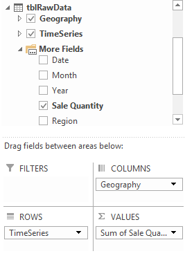
Image 5: PivotTable field settings with Hierarchy fields
Step 10: Click on + sign in PivotTable report to expand the hierarchy.
Step 11: Finally after few pivot design editing the report will looks like below:

Image 6: Final view of a sales report by using Hierarchy field
The findings is, if we used normal fields for report generating, then we need to use few fields individually in ROWS and COLUMNS section. But to get the same result, if we use Hierarchy fields, then we can generate the same report in short time.