
New Article

How to SUM by matching partial text in Excel

What is Array Formula?

Do you want to be an Excel Power User? Then no other choice left except learning Array Formulas. An Array Formula can calculate your desire result faster and easy way that you can't do by using regular formula. Array Formula always ends with Ctrl+Shift+Enter while a Regular Formula ends with a single Enter. After pressing Ctrl+Shift+Enter you will see "{" "}" curly brackets are added in the starting and ending point of your formula. That is why it is also known as CSE Formula.


Why you should use array formulas?

If you have experience of using non-array formula, then I can say, you are able to calculate few things like Daily Sales Growth, Sales Forecasting, ROI (Return of Investment) etc. However if you really want to become an expert user of Microsoft Excel, then you must know Array Formulas. Array Formula is like magic power to get the desire result.


What is Array?

An Array means a set of items. More clearly, an Array is a range in Excel formula that contains items. If you are looking for an item which is in the range, it returns TRUE if it matched.

Transpose() is a simple example of Array Formula. You can convert data from Row to Column through this function.


Image 1: Array formula

Another example is SUMPRODUCT(). SUMPRODUCT() is simply used to multiply 2 rows or columns. In the example below A1:A10 and D1:D10 is the data range. If you use the SUMPRODUCT() simply use:

=SUMPRODUCT(A1:A10,D1:D10)

This will show the result 110. On the other hand you can use SUM function to do the same thing. After using the CSE command the Array formula looks like:

{=SUM(A1:A10*D1:D10)}

And the result is same 110.


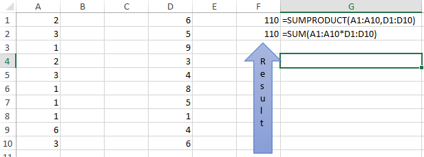
Image 2: SUM as array formula

Remember one thing:

Popular posts from this blog

How to display an image in worksheet based on a List or based on IF condition?

Excel can show image on worksheet based on a specific IF condition. So, how to do it? Simple follow the below steps: Step by Step: Step 1: Insert images in your Excel Worksheet. Here I've inserted 5 different types of balls, Football, Cricket, Pool, Basketball, Tennis ball. Note that, All balls are placed into different cell. These are placed in Picture sheet. Image 1: 5 balls placed in 5 different cells and covered photo's wide and height Step 2: In the report sheet, design the report as you wish. I've designed in my way like below: Image 2: Kids asking to Donald Duck, which ball need to throw now Step 3: Make a drop down list "Games" in E6 cell in Report sheet from Data Validation. which is as below: Football Cricket Pool Basketball Tennis You can do an IF function here in E6 in Report sheet, which will meet a certain condition and returned Football, Cricket, Pool, Basketball or Tennis. Step 4: Now the tricky part is

Fiverr Microsoft Excel 2016 Skill Test and Answers 2021

This video will help you about preparing Fiverr Excel Skill Test. I've just taken this Fiverr Excel Skill Test and successfully passed with a scored 6 out of 10. I'm sharing my Fiverr Excel Skill Test and Answers 2021 video so that you can prepare yourself if you would like to give a test on Fiverr.    I have taken the Fiverr Excel Skill Test on Fiverr and obtained 6 out of 10 scores. If you take a test and pass, it will greatly help the buyer to trust you and your skills. Please note that your exam will not be exactly the same as mine because there are many more questions in the pool than 40 which appeared in my test. But I am hopeful that you will succeed in it. If you have any queries, please write them in the comment section. I will try my best to guide you.Follow this video and try to get a general idea. By following the instructions, you can successfully pass the test.    After passing the Fiverr Excel Skill Test, Fiverr shared a Excel Expert Badge on my Profile, so that

Cumulative Closing Balance like a Bank Statement in PivotTable

A Bank Employee in many case needs to calculate the Closing Balance after each transaction in PivotTable like a Bank Statement . But with the help of Calculated Field of a PivotTable , you can only calculate Field with Field . It's not possible to use a formula in Calculated Field where you can mention a single cell with Relative Reference Cell . Because a PivotTable acts like a Table format where you can work with Field or Column Name . A Helping Column (A regular column, that helps to get a partial result where formula applied) can be a good idea. But there is an option in PivotTable by which you can Calculate Cumulative . In this article I will show you, how you can do it. Calculating with Formula: Assume that, you have an Excel file with Debit and Credit transaction of an Account . Image 1: Sample Bank Statement In a Bank Statement , Month wise Cumulative Balance is important. In the Excel sheet, as above, it is very easy to use a formula and calc