This is the first report I'm going to prepare through Power BI Desktop. The first thing is adding raw data. To do this, you need to Click the Get Data option in Startup Screen.

If you are advanced user, then you don't need to open this startup window all the time while you need to open data sources. You can get data by Clicking on Home | Get Data | More.
While the Get Data dialog box appeared, Select the Excel program and Click on Connect button:

After appearing Open dialog box, Select the Excel file which you want to open and Click on Open button.
Now this will connect to your Excel file. When it is done, it will show you a Navigator dialog box listed with all data tables present in that Excel file. Select the Table or Tables which you want to open (i.e. Invoice) and Click on Load.
After Loading, it will show you Sheet Names. If you have 2 different tables in 1 Sheet, then Convert each table to Table format by Selecting and Pressing Ctrl+T+Enter. If you Select any Sheet then it will show you a preview:


Now to do your first report just Click the Chart type to Select it from Visualization Pane and then drag and drop the Category field from Fields Tab to Report Tab. This will add the Category in Report View tiles. Again drag and drop the QTY field from Fields Tab to Report Tab.
The default view of the Power BI Desktop is called Report View. There are 5 different areas of Report view:

Now Save the report by Clicking on File | Save. For the first time saving, type a name PBD_01 and Click on Save. This will save the file as PBD_01.pbix.
After successfully published the Report to Power BI Service (on the web), this will show you a dialog box.

Now if you want to see this report in Power BI Service to check it, then Click on Open 'PBD_01.pbix' in Power BI link. This will open the Power BI Service in your Web Browser.

Click on the Pin Visual icon of the Histogram Chart in Power BI Service to Pin the report nicely and generate the Dashboard for viewing.

After Clicking the Pin visual, this will appears a dialog box Pin to Dashboard. For the first time, by default New Dashboard option has already Selected. Type a name Pin01 and Click on Pin.
To view the Dashboard, Click on the Show the Navigation Pan from the left side. Then Click on My Workspace and Select Dashboard. And then Click the Dashboard Name to view the Dashboard.

By this way you can view your generate your reports in Power BI Desktop and publish it to Power BI Service and can read it through Power BI Mobile. But before viewing on your Windows Phone, make sure that, your OS of Windows Phone is Windows 10. Windows 8.1 will not support this apps.
Now you can play with your Charts. For example. If you generate 2 Reports like below, and Click on Bagherhat histogram bar:

Then in Map your sales data also filtered:


Image 1: Startup Screen of Power BI Desktop
If you are advanced user, then you don't need to open this startup window all the time while you need to open data sources. You can get data by Clicking on Home | Get Data | More.
While the Get Data dialog box appeared, Select the Excel program and Click on Connect button:

Image 2: Get Data dialog box
After appearing Open dialog box, Select the Excel file which you want to open and Click on Open button.
Now this will connect to your Excel file. When it is done, it will show you a Navigator dialog box listed with all data tables present in that Excel file. Select the Table or Tables which you want to open (i.e. Invoice) and Click on Load.
After Loading, it will show you Sheet Names. If you have 2 different tables in 1 Sheet, then Convert each table to Table format by Selecting and Pressing Ctrl+T+Enter. If you Select any Sheet then it will show you a preview:

Image 3: Preview of Invoice Sheet
Image 4: All data of Invoice Sheet have loaded in Power BI Desktop
Now to do your first report just Click the Chart type to Select it from Visualization Pane and then drag and drop the Category field from Fields Tab to Report Tab. This will add the Category in Report View tiles. Again drag and drop the QTY field from Fields Tab to Report Tab.
The default view of the Power BI Desktop is called Report View. There are 5 different areas of Report view:

Image 5: Areas of Power BI Desktop
Now Save the report by Clicking on File | Save. For the first time saving, type a name PBD_01 and Click on Save. This will save the file as PBD_01.pbix.
Remember that, Power BI is a collection of software, Services and Apps. You will generate your reports to Power BI Desktop, then publish it to Power BI Service on the web and finally you can view your reports from Power BI Mobile Apps.Click the Publish button from the Home menu to publish the report to Power BI on the Web.
After successfully published the Report to Power BI Service (on the web), this will show you a dialog box.
Image 6: Successfully Published to Power BI
Now if you want to see this report in Power BI Service to check it, then Click on Open 'PBD_01.pbix' in Power BI link. This will open the Power BI Service in your Web Browser.
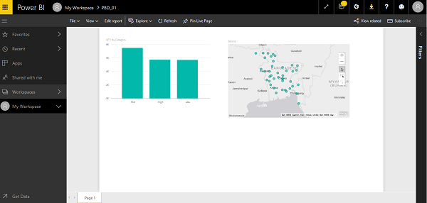
Image 7: Published the Report in the web (Power BI Service)
Click on the Pin Visual icon of the Histogram Chart in Power BI Service to Pin the report nicely and generate the Dashboard for viewing.

Image 8: Pin visual
After Clicking the Pin visual, this will appears a dialog box Pin to Dashboard. For the first time, by default New Dashboard option has already Selected. Type a name Pin01 and Click on Pin.
To view the Dashboard, Click on the Show the Navigation Pan from the left side. Then Click on My Workspace and Select Dashboard. And then Click the Dashboard Name to view the Dashboard.

Image 9: Viewing Dashboards
By this way you can view your generate your reports in Power BI Desktop and publish it to Power BI Service and can read it through Power BI Mobile. But before viewing on your Windows Phone, make sure that, your OS of Windows Phone is Windows 10. Windows 8.1 will not support this apps.
Now you can play with your Charts. For example. If you generate 2 Reports like below, and Click on Bagherhat histogram bar:

Image 10: Another Dashboard
Then in Map your sales data also filtered:

Image 11: Filtered Map data
Similarly if you can Click the Sales Circle of any one in the Map, then Histogram of that Sales data will activated.