Scenario is very helpful tool in Excel for Data Analysis. Not only in our professional life but also it can be used in our personal life. It helps to get the perfect decision for your problems. This is the secret of the Scenario tool. Now let's start working and destroy your problems.
The Problem:
Assume that, you want to purchase 30 units of Smart Phones for your own business. The unit price is 11000 BDT. The Carrying Cost, VAT and others cost in total 2500 BDT. So, you have invested for your business is total 332500 BDT. (30 * 11000 = 330000 BDT + 2500 BDT). Now you need to take a decision about "what will be the Sell-Out price per unit of your product to earn a suitable profit?".
In Excel sheet plot this problem like below:

In E3 cell the formula is =D3*C3. F3 cell contains an amount fixed 2500. Total Invested Amount in G3 cell =E3+F3. In I3 cell the formula is =H3*C3 and in J3 cell the formula is =I3-G3.
Scenario Manager:
This problem can be solved through Goal Seek if you know the Total Profit Amount. But as discussed above I would like to go with Scenario, which will help me to set different Sell-Out Price (Per Unit) and whatever I want I can see the Total Profit based on this.
But before starting, I want to say, you can work with more than 1 custom Scenario values to see the changes. Here I have used only a single cell H3 so that you can easily understand the Scenario. If you want you can use more than 3 cells based on your calculation dependent cells to see the Scenario.
So, let's start:
Step 1:
Click on Data | What-If Analysis | Scenario Manager. Then a dialog box will appear.

Step 2:
Click on Add button. This will appear a dialog box like below image:

In the Scenario name enter a name so that you can easily understand what value you have entered in Changing cells. Here I will analyze through the Sell-Out unit price which will start from 11000 BDT. So I am going to enter S/O Price 11000. And in Changing cells I would like to enter H3 cell because it is the cell where I need to enter Sell-Out Unit Price.
Notice that, if your calculation depends on 2 or more cell values and need to changes, then you can use Red Collapse button and Press and Hold CTRL key and Click the cells where you want to change values.

Keep the Protection options as it is and then Click on Ok button. The Scenario Values dialog box will appear:

This dialog box asking you, what value you want to post in H3 cell. Remember you entered a name with 11000 BDT. So Value will be here in H3 is 11000. Enter 11000 in this dialog box and Click on Ok.

If you selected many cells, you will see 1:, 2:, 3:, text boxes in Image 6. I've selected only one cell to change, so 1: is appeared. If you wish more then it, you can see Cell NAME instead of $H$3 in Image 6. But to do this, you need to Select the Cell H3 and Name it from the Name Box. Just like below:

Click on Ok. Now you will back to the Scenario Manager dialog box. And this time this will looks like below:

Step 3:
In this way, you can add few more data in Scenario Dialog box by Clicking on Add button like below image:

Step 4:
Now time to see the result. Click on any Scenarios and Click on Show button. Suppose I would like to see what happens when I choose 12500 BDT. as Sell-Out unit price. To do this just double Click on S/O Price 12500 or Click on S/O Price 12500 and then Click on Show button to see the result in Calculation Table like below image:

By this way you can watch which S/O Price would be perfect for gaining suitable profit. Here suitable profit mean not too High not too Low. If you want to edit some Scenarios items simply Select that item under Scenarios box and Click on Edit button. Also you can Delete unnecessary Scenarios from here. I think a little briefing needs for Merge option.
How to Merge Scenario?
Merging Scenario means, importing Scenarios from outside, like others Sheets within the same Workbook or others Workbooks. Here I would like to explain how you can Merge (Import) Scenarios from others Sheet within the same Workbook. Assume that, you have all the above Scenarios in Sheet1. And in Shee2, you have below Scenarios:

Now what I'm going to do is, Import these 3 Scenarios from Sheet2 to Sheet1 where I've Calculated a Profit/Loss. To Merge Scenarios from Sheet2 to Sheet1 please follow below instructions:
- Click on Sheet1 and then Click on Data | What-If Analyze | Scenario Manager. A dialog box will appear like below image:

Notice that, the dialog box offers you to choose Book: and Sheet name. And above OK button there is a small information said: "There are 3 scenarios on source sheet". This means that, the Shee2 has already 3 new Scenarios. If you Select the Sheet2 and Click on Ok, then all of these 3 Scenarios will import into Sheet1. But don't worry, it will not moved, just copied.
- Select Sheet2 and Click on Ok. Now the dialog box will looks like below after imported 3 new Scenarios into Sheet1:

If you Select Term 30 and Click on Show button, then the value of Term 30 will show in $C$5 in Sheet1 as set.
How to view Summary Report?
Scenario Manager dialog box allows you to view each Scenarios Result at a glance in Excel worksheet through Scenario Summary and through Scenario PivotTable Report. First I will discuss about Scenario Summary and then Scenario PivotTable Report.
Scenario Summary:
Scenario Summary will shows all the saved Scenario result in a New Excel Sheet. To view this just Click on Summary button. This will appear a dialog box like below:
- Select Scenario summary option from Report type.
- Then Click the cell based on which you want to view the report. As I've analyzed Sell-Out Price (Per Unit), but result shown in J3, so I have selected J3 cell in Result cells. And then Click on Ok. This will show a Summary Report like below image:
This report said that, Changing Cells when 12500 BDT. then Result Cells (Profit 42500). And by this way from D to I column the result shows. You can choose the best profit package from here. The J to L column is from others Scenario which have imported from Sheet2. These are not related with Profit calculation. So, you can clear these columns.
Scenario Pivot Table Report:
This option will allows you to view the summary report of all your Scenarios through PivotTable like below image:

Notice that, all the fields in PivotTable are selected automatically. So, you don't need to drag and drop manually.
So, by this way you can use Scenario Manager to take your decisions. You can apply changing cells 3 or more for calculation. Hope this important tool is now clear to all of you.
|||| Please SUBSCRIBE our YouTube Channel ||||
https://www.youtube.com/channel/UCIWaA5KCwZzBGwtmGIOFjQw
The Problem:
Assume that, you want to purchase 30 units of Smart Phones for your own business. The unit price is 11000 BDT. The Carrying Cost, VAT and others cost in total 2500 BDT. So, you have invested for your business is total 332500 BDT. (30 * 11000 = 330000 BDT + 2500 BDT). Now you need to take a decision about "what will be the Sell-Out price per unit of your product to earn a suitable profit?".
In Excel sheet plot this problem like below:

Image 1: Problem plotting
In E3 cell the formula is =D3*C3. F3 cell contains an amount fixed 2500. Total Invested Amount in G3 cell =E3+F3. In I3 cell the formula is =H3*C3 and in J3 cell the formula is =I3-G3.
Scenario Manager:
This problem can be solved through Goal Seek if you know the Total Profit Amount. But as discussed above I would like to go with Scenario, which will help me to set different Sell-Out Price (Per Unit) and whatever I want I can see the Total Profit based on this.
But before starting, I want to say, you can work with more than 1 custom Scenario values to see the changes. Here I have used only a single cell H3 so that you can easily understand the Scenario. If you want you can use more than 3 cells based on your calculation dependent cells to see the Scenario.
So, let's start:
Step 1:
Click on Data | What-If Analysis | Scenario Manager. Then a dialog box will appear.
Image 2: Scenario Manager dialog box
Step 2:
Click on Add button. This will appear a dialog box like below image:
Image 3: Add Scenario dialog box
In the Scenario name enter a name so that you can easily understand what value you have entered in Changing cells. Here I will analyze through the Sell-Out unit price which will start from 11000 BDT. So I am going to enter S/O Price 11000. And in Changing cells I would like to enter H3 cell because it is the cell where I need to enter Sell-Out Unit Price.
Notice that, if your calculation depends on 2 or more cell values and need to changes, then you can use Red Collapse button and Press and Hold CTRL key and Click the cells where you want to change values.

Image 4: Adding a Scenario
Keep the Protection options as it is and then Click on Ok button. The Scenario Values dialog box will appear:
Image 5: Scenario Values dialog box
This dialog box asking you, what value you want to post in H3 cell. Remember you entered a name with 11000 BDT. So Value will be here in H3 is 11000. Enter 11000 in this dialog box and Click on Ok.
Image 6: Entered Scenario Values
If you selected many cells, you will see 1:, 2:, 3:, text boxes in Image 6. I've selected only one cell to change, so 1: is appeared. If you wish more then it, you can see Cell NAME instead of $H$3 in Image 6. But to do this, you need to Select the Cell H3 and Name it from the Name Box. Just like below:
Image 7: Name used instead of $H$3
Click on Ok. Now you will back to the Scenario Manager dialog box. And this time this will looks like below:
Image 8: 1 data added in Scenario Manager
Step 3:
In this way, you can add few more data in Scenario Dialog box by Clicking on Add button like below image:
Image 9: Added few more data in Scenario Manager
Step 4:
Now time to see the result. Click on any Scenarios and Click on Show button. Suppose I would like to see what happens when I choose 12500 BDT. as Sell-Out unit price. To do this just double Click on S/O Price 12500 or Click on S/O Price 12500 and then Click on Show button to see the result in Calculation Table like below image:

Image 10: Scenario Manager Shows the Scenario Value in H3 cell and I3 and K3 shows the result as formula already entered there
By this way you can watch which S/O Price would be perfect for gaining suitable profit. Here suitable profit mean not too High not too Low. If you want to edit some Scenarios items simply Select that item under Scenarios box and Click on Edit button. Also you can Delete unnecessary Scenarios from here. I think a little briefing needs for Merge option.
How to Merge Scenario?
Merging Scenario means, importing Scenarios from outside, like others Sheets within the same Workbook or others Workbooks. Here I would like to explain how you can Merge (Import) Scenarios from others Sheet within the same Workbook. Assume that, you have all the above Scenarios in Sheet1. And in Shee2, you have below Scenarios:

Image 11: Scenarios in Sheet2
Now what I'm going to do is, Import these 3 Scenarios from Sheet2 to Sheet1 where I've Calculated a Profit/Loss. To Merge Scenarios from Sheet2 to Sheet1 please follow below instructions:
- Click on Sheet1 and then Click on Data | What-If Analyze | Scenario Manager. A dialog box will appear like below image:
Image 12: Merge Scenarios
Notice that, the dialog box offers you to choose Book: and Sheet name. And above OK button there is a small information said: "There are 3 scenarios on source sheet". This means that, the Shee2 has already 3 new Scenarios. If you Select the Sheet2 and Click on Ok, then all of these 3 Scenarios will import into Sheet1. But don't worry, it will not moved, just copied.
- Select Sheet2 and Click on Ok. Now the dialog box will looks like below after imported 3 new Scenarios into Sheet1:
Image 13: Imported new 3 Scenarios
If you Select Term 30 and Click on Show button, then the value of Term 30 will show in $C$5 in Sheet1 as set.
How to view Summary Report?
Scenario Manager dialog box allows you to view each Scenarios Result at a glance in Excel worksheet through Scenario Summary and through Scenario PivotTable Report. First I will discuss about Scenario Summary and then Scenario PivotTable Report.
Scenario Summary:
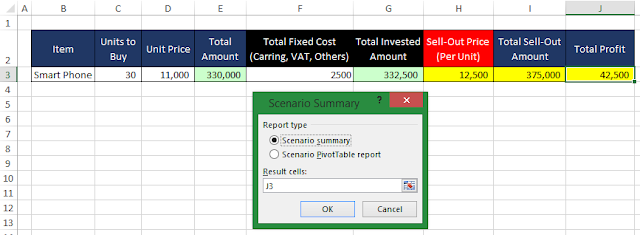
Scenario Summary will shows all the saved Scenario result in a New Excel Sheet. To view this just Click on Summary button. This will appear a dialog box like below:

Image 14: Scenario Summary
- Select Scenario summary option from Report type.
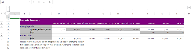
- Then Click the cell based on which you want to view the report. As I've analyzed Sell-Out Price (Per Unit), but result shown in J3, so I have selected J3 cell in Result cells. And then Click on Ok. This will show a Summary Report like below image:

Image 15: Scenario Summary
This report said that, Changing Cells when 12500 BDT. then Result Cells (Profit 42500). And by this way from D to I column the result shows. You can choose the best profit package from here. The J to L column is from others Scenario which have imported from Sheet2. These are not related with Profit calculation. So, you can clear these columns.
Scenario Pivot Table Report:
This option will allows you to view the summary report of all your Scenarios through PivotTable like below image:

Image 16: Scenario PivotTable Report
Notice that, all the fields in PivotTable are selected automatically. So, you don't need to drag and drop manually.
So, by this way you can use Scenario Manager to take your decisions. You can apply changing cells 3 or more for calculation. Hope this important tool is now clear to all of you.
|||| Please SUBSCRIBE our YouTube Channel ||||
https://www.youtube.com/channel/UCIWaA5KCwZzBGwtmGIOFjQw