Converting any TEXT (actually numerical value but in TEXT mode) value to NUMBER or from NUMBER to TEXT is a daily routine in Excel. Many array formulas while you are trying to Lookup a Numerical Value but actually that was in TEXT mode, you need to convert your Lookup value first and then start lookup. Sometimes reverse of it. So, if you are facing this problem, then learn this trick which you help you a lot in Excel Calculation.
Convert TEXT to NUMBER:
There are 2 main ways to convert a Text value to Number. These are:
(a) Use "+0" after formula:
After removing extra spaces or took the number with LEFT, RIGHT, MID etc command, use a "+0" (Plus Zero) at the end of the formula immediately. For Example:

(b) Use VALUE():
This is another way to converting a Text numerical value to Calculative numerical value. Use this VALUE() within the entire formula. For Example:

If this VALUE() failed to convert it, then you will get a #VALUE error. Make sure there is no Alphabetical characters in your Text value. If found then try to remove with TRIM(), CLEAN() or SUBSTITUTE().
Convert NUMBER to TEXT:
Sometimes you need to convert a Number to a Text value. For example, you may need to mention a value with reference cell which is a Numerical Value but actually it is in Text mode. Then you can try below examples:
(a) Add '&""" after the number:
By Adding a blank character at the end of the Number can convert a Number to Text.

(b) Apply TEXT():
By using the Text function you can also convert the Number to Text:
Convert TEXT to NUMBER:
There are 2 main ways to convert a Text value to Number. These are:
(a) Use "+0" after formula:
After removing extra spaces or took the number with LEFT, RIGHT, MID etc command, use a "+0" (Plus Zero) at the end of the formula immediately. For Example:
Image 1: Using "+0" formula
(b) Use VALUE():
This is another way to converting a Text numerical value to Calculative numerical value. Use this VALUE() within the entire formula. For Example:
Image 2: VALUE()
If this VALUE() failed to convert it, then you will get a #VALUE error. Make sure there is no Alphabetical characters in your Text value. If found then try to remove with TRIM(), CLEAN() or SUBSTITUTE().
Convert NUMBER to TEXT:
Sometimes you need to convert a Number to a Text value. For example, you may need to mention a value with reference cell which is a Numerical Value but actually it is in Text mode. Then you can try below examples:
(a) Add '&""" after the number:
By Adding a blank character at the end of the Number can convert a Number to Text.
Image 3: Adding a "&"""
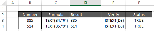
(b) Apply TEXT():
By using the Text function you can also convert the Number to Text:
Image 4: Applying TEXT()