Battery Chart is a great way to view the percentage information. It can easily represent many reports with "Still Remaining" information. Such as, The remaining achievement value, the remaining achievement percentage, the remaining days to go in this month etc. This chart can attract audience in seconds. So, using of this chart could be a plus point of your professional career.

Image 1: Battery Chart in Excel
Understanding A Battery Chart:
To create a Battery Chart, first of all I divide a battery into 4 parts. Bottom Portion, Achievement Value, Remaining Value and Top Portion. To design a Battery Chart I also need to divide a single information into 4 parts.
Data Require to Create a Battery Chart:
If I have a single information like, Achievement Percentage is 63%, then I can find another information like, 100% - 63% = 37%. So I can call it, Achievement Value = 63% and Remaining Value = 37%. Manually I have selected The Bottom Portion = 2% and Top Portion = 2%. Here the value of Top and Bottom Portion are completely not calculating with Value and Remaining Value. It is separated and just set to view the battery chart good. It can be set to 3%, 2.5% or 1% etc.

Remember that, Achievement Value and Remaining Value equals to your Total Target Value. The Bottom and Top Values are only for designing your Battery Chart, nothing else.
Now if you plot this calculation in an Excel sheet then it will looks like below:

Image 2: Data require to create a Battery Chart
Steps to Create a Battery Chart:
Step 1:
Select B2:C5 cell and Click on Insert ➪ Chart ➪ Insert Column or Bar Chart ➪ 3D-Stacked Bar. Now convert this Bar Chart to Column Chart by Clicking the Switch to Row/Column button from Design Tab. Make sure that, the inserted chart must be selected. Otherwise the Design Tab will not shows in Menu bar.
Select B2:C5 cell and Click on Insert ➪ Chart ➪ Insert Column or Bar Chart ➪ 3D-Stacked Bar. Now convert this Bar Chart to Column Chart by Clicking the Switch to Row/Column button from Design Tab. Make sure that, the inserted chart must be selected. Otherwise the Design Tab will not shows in Menu bar.
Step 2:
Right Click on any Bar in the chart and Click on Format Data Series. This will show a Format Data Series task pane. Click on Cylinder radio button and Select Gap Width 0% and Gap Depth as 0% like below image:

Image 3: Cylinder Bar and Gap Width and Depth 0%
Step 3:
Click on Chart Elements button and Uncheck all the option, like Axis, Axis Title, Legend etc.
Step 4:
Set the Fill Color as Solid color and Select the same color (Gray) for Top Portion and Bottom Portion. Set the same deep color for Achievement Value and Remaining Value. Please note that, the color of Achievement Value and Remaining Value must be same color and it should be deep color.

Image 4: Color Selection
Step 5:
Now Select the Remaining Value bar and Set the Transparency as 78% (in my opinion, if you wish you can set as you like best).
Image 5: Transparency 78%
Step 6:
For the final drawing, Insert a Flowchart: Direct Access Storage from Insert ➪ Auto Shape and place it after the Top Portion. This will looks like Carbon cylinder bar of a battery.
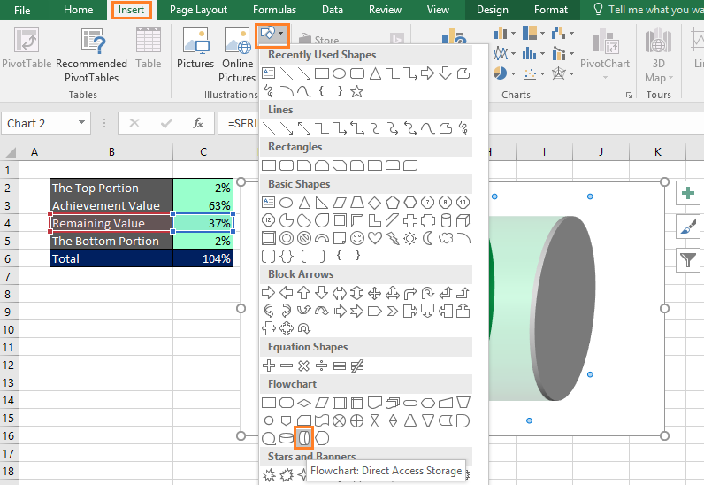
Image 6: Carbon Cylinder of Battery
Step 7:Finally Select Chart, then from Format Plot Area task pane, Select 3D Rotation and Set X Rotation 13 and Y Rotation 0. Now Right Click on the Achievement Value and Select Add Data Label ➪ Add Data Labels. After a resizing with Mouse the final Battery Chart will looks like this:

Image 7: Battery Chart
|||| Please SUBSCRIBE our YouTube Channel ||||
https://www.youtube.com/channel/UCIWaA5KCwZzBGwtmGIOFjQw
|||| Please SUBSCRIBE our YouTube Channel ||||
https://www.youtube.com/channel/UCIWaA5KCwZzBGwtmGIOFjQw