Learn How to Use AutoFill in Excel to Save Time on Worksheet

In Excel, you often work with a data table for data analysis. While working on data table, you my need to populate your data table through importing or manually entering them which is called data typing. It is true that, this will take time. But do you know that, there are few features in Excel which allows you to auto fill up your data table?. Yes, there are few features available in Microsoft Excel which allows you to auto fill your data table and save time while working on worksheet. Such as, One Input Data Table, Two Input Data Table, Goal Seek, AutoFill etc.

 

In this lesson, I'll help you to learn how to use AutoFill in Excel and save your time. It is very simple to use. Just a double click you need to do it. AutoFill is really a powerful tool in Microsoft Excel. It will populate your data table in seconds and save your time while working on worksheet.

 

AutoFill is a great feature in Microsoft Excel which allows you to fill series of numbers, dates and other data, create and use a custom lists. It will fill up to down or left to right with data automatically. It is very easy to use and you can use it quickly.

 

 

Use AutoFill for Different Data Types in Excel:

Using of AutoFill feature is completely depends on your data type and requirements. You can apply AutoFill Numbers for below data table in different ways in Excel:

1. Autofill a Series of Numbers:
 

There are different types of number on which you can apply AutoFill function. These are:

A. Data Related to Numbers:
 

This is very simple. It is 1, 2, 3, 4 and goes on. For example if you have an excel worksheet contains 13 Names and you want to make it a list by adding another column besides this column and make a serial, then follow below steps:

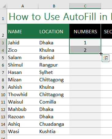
Step 1: Type 1 in C3 cell and 2 in C4 cell.
Step 2: Then Select the C3:C4 cell. You will see a small square box visible (it always visible when you are not in cell editing mode). This is called Fill Handle.
Step 3: Place your cursor on Fill Handle. You will see the cursor changed to a Plus ('+') symbol.

 

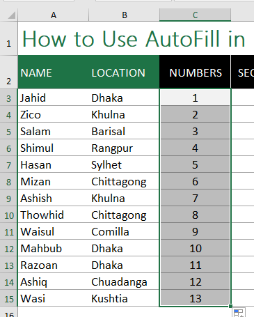
Step 4: Left Click on it and hold the Click (if you are right handed mouse user) then drag it down. You will see a magic. It automatically filled the serial in seconds.

Tips:
Autofill through Mouse Dragging allows Fill Up besides Fill Down. Example: 2, 1, 0, -1, -2 and goes on.

If you are unable to apply Mouse Dragging, then Excel has an alternative ways to use Autofill. To do this follow the below steps:

Step 1: Select C3:C15 cell range.
Step 2: Click on Home | Fill | Series.
Step 3: Series dialog box will appear.

 

Step 4: Select Columns from "Series in" section as you are trying to filling down automatically, within a column.
Step 5: Select AutoFill from Type.
Step 6: Click on Ok.

Tips:
In Step 5, you can also Select Linear and set the Step Value 1 in the dialog box and Click on Ok.

B. Data That Not Related to Numbers:
 

If the data is not related with numbers, it also can autofill. For example, if you have an excel worksheet contains 2 Items "First Name 1" in D3 cell and "Last Name 1" in D4 cell and you want to make it a list down by adding more "First Name 2" and "Last Name 2" for 13 different person, Excel can do it. Although it is not a proper number, but it can automatically fill if you drag it. To do this follow the below steps:

Step 1: Select D3:D4 cell.
Step 2: Simply drag your mouse down like previous.

Now can you see that, it automatically filled the serial in seconds? It's very powerful tool.

C. Even Numbers:

Not only Microsoft Excel can fill automatically serial numbers, it can also be able to fill Even Numbers. For example if E3 = 2 and E3 = 4, then follow the below steps:

Step 1: Select E3:E4.
Step 2: Drag your mouse down.

 

 

It will auto fill 2, 4, 6, 8 etc all even numbers.

 

 

D. Odd Numbers:
 

It can also be able to fill odd numbers. For example if F3 = 1 and F4 = 3, then follow the below steps:

Step 1: Select F3:F4.
Step 2: Drag your mouse down.

 

It will auto fill 1, 3, 5, 7 etc all odd numbers.

 

 

E. Sequence Numbers:

You can solve puzzle questions through AutoFill like "What will be the next number". For example if G3 = 7, G4 = 10 and G5 = 16, then follow the below steps:

Step 1: Select G3:G5.
Step 2: Drag your mouse down.

 

It will auto fill 7, 10, 16, 20, 24.5, 29, 33.5, 38 etc.

 

2. Autofill Dates:
 

Not only AotuFill can automatically fills Numbers, but also it can autofills Days, Dates, Weekdays, Months, Years.

A. Autofill Dates:

If H3 = 5-Nov-21 then follow the below steps:

Step 1: Select H3 cells only.
Step 2: Drag your mouse down.

 

It will autofill 5-Nov-21, 6-Nov-21, 7-Nov-21, 8-Nov-21 etc.

Tips:
You can also do this by selecting H3:H15 cells and Select Linear from Type and set Step value as 1.

B. Autofill Day:

If I3 = Fri, then follow the below steps:

Step 1: Select I3 cells only.
Step 2: Drag your mouse down.

 

It will autofill Fri, Sat, Sun, Mon etc.

C. Autofill Month:

If J3 = Jan, then follow the below steps:

Step 1: Select J3 cells only.
Step 2: Drag your mouse down.

It will autofill Jan, Feb, Mar, Apr etc.

3. Autofill Formulas:

AutoFill can also be fill down your formulas. If K3:K10 contains =COUNTIF($B$3:B3,B3) formula and you need to copy down the formula where cell will automatically changed within the column, then do the following:

Step 1: Select K3 cell and Drag your Mouse.

Tips:
Use Ctrl + D Shortcut command for formula copy down in Microsoft Excel.

4. Autofill Cell Formatting:

Autofill can fills automatically cell formatting. For example, if L3 cell is Bold and Fill Color Red, Font Color White. And you need to copy down this cell formatting then do the following:

Step 1: Select L3:L15
Step 2: Press Ctrl + D

 

Tips:

If you apply Ctrl + D, then cell Formatting or Formula will copy down. But if you use Mouse Drag then it will keep all including Autofill Numbers, Dates and others.

5. Autofill on Filtered Data

 

Autofill also supports on Filtered data. For example, if M3:M15 = 15-Nov-21 to 19-Nov-21 and you have already applied a filtered (visible rows) on 16-Nov-21 and 18-Nov-21, and you want to apply a Autofill for only M3 and M5 cell, then do the following:

Step 1: Select M3:M15

Step 2: Apply Filter by pressing Ctrl + Shift + L.
Step 3: Select 16-Nov-21 and 18-Nov-21.

Step 4: Apply a Fill color (for example yellow) in M3 cell.

Step 5: Drag your Mouse down.

The result will be like below image:

Now if you release the filter, then you will see that, others cell are not filled by yellow color. Than means Excel Autofill can also be use on filtered only data.

6. AutoFill with A Custom List
 

Yes, you can create your own custom AutoFill list. For example if you want to create a custom list "A, B, C, D to Z" which is like others already created in Microsoft Excel default list "Jan, Feb, Mar" or "Sat, Sun, Mon", then follow below steps:

Step 1: Click the File tab choose Options, Advanced tab, scroll down to the General section, then click the Edit Custom Lists button.

 

 
Step 2: Custom Lists dialog box will appear.

Step 3: Click on New List from Custom lists option. A cursor will appear in List entries section.

 

Step 4: Type values with Comma (,) to separate cell value. Type A, B, C, D, E, F, G, H, I, J, K, L, M, N, O, P, Q, R, S, T, U, V, W, X, Y, Z.

 

Step 5: Click on Add button. It has now created and will show in Custom Lists box.

 

Step 6: Click on Ok.

To apply this Custom List, type A in N2 cell. Select the N2 cell and copy down. See the magic. By this way you can add many more of your own list. Don't worry, you can delete the unnecessary custom list.

Trouble Shooting about AutoFill Not Working:

1. Alphabetical letters are keep repeating, not working:

In Microsoft Excel, there are some default custom lists. These are:
(a) Jan, Feb
(b) Fri, Sat
(c) January, February
(d) Friday, Saturday

If you try outside of this custom alphabetical list, then Microsoft Excel will unable to help you automatically fill up your requirements. To do this you need to add them first. Please follow our How to add a Custom List in Microsoft Excel tutorial section in this article to add your missing Custom list.


2. While I place my Mouse Pointer over Fill Handle (small autofill square), it is not changed to "+" symbol and I'm unable to use AutoFill:

If your Mouse Pointer is not changing to "+" symbol, then you can Enable it by following below steps:

Step 1: Click on File | Options | Advance
Step 2: In the Editing options section, Check "Enable fill handle and cell drag-and-drop.

This will enable the "+" symbol for your AutoFill.

Video Tutorial: