Remove duplicate values but keep one value:
So, In Microsoft Excel when you start data analysis based on one column, it is very important to keep your data clean and must follow the data table rules. Otherwise your query on data table will show you wrong result. One of the data table rule is, every record or row will be unique based on one column. In Microsoft Excel you can check and remove duplicate values or rows based on one column. This feature in Microsoft Excel is called Remove Duplicate. It is a built-in tool of Microsoft Excel which helps you to clean up your data quickly. It is very easy to use.
In this tutorial I'll show you how you can remove duplicates rows in excel and keep first record or row only from each duplicate records or rows based on one column.
How to use Remove Duplicate in Excel 2016
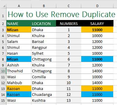
Let's start with a simple example here. Below is a data table where few columns contains duplicate values. We can remove these duplicate values but keep the first value based on one column or based on multiple columns.
Use Remove Duplicate for Single Column:
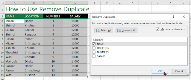
There are duplicate values in Name column. So, if we want to remove duplicate names and keep the first record only, then follow below steps:
1. Click anywhere of the data table.
2. Click on Data | Remove Duplicates.
3. Remove Duplicates dialog box will appear.
4. Click on Unselect All.
5. Check on Name
6. Click Ok.
Tips:
Make sure that, "My data has headers" option in "Remove Duplicates" dialog box checked. Otherwise you have to identify with Column Number like Column 1, Column 2 etc.
Microsoft Excel will notify you with a message that, how many duplicate values found and removed, also how many unique values remain in Name column.
Use Remove Duplicate for Multiple Columns:
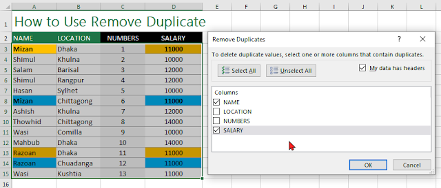
If there is a criteria that, if Name and Salary is same value for a single record, then it is must be a duplicate. So you have to keep first and delete others same record. To do this, follow the instructions:
1. Click anywhere of the data table.
2. Click on Data | Remove Duplicates.
3. Remove Duplicates dialogbox will appear.
4. Click on Unselect All.
5. Check on Name and Salary
6. Click Ok.
Microsoft Excel will notify you with a message that, how many duplicate values found and removed, also how many unique values remain in Name column.
How many ways you can identify duplicate values in Excel 2016:
There are 2 ways you can identify the duplicate records. These are:
A) Through Conditional Formatting:
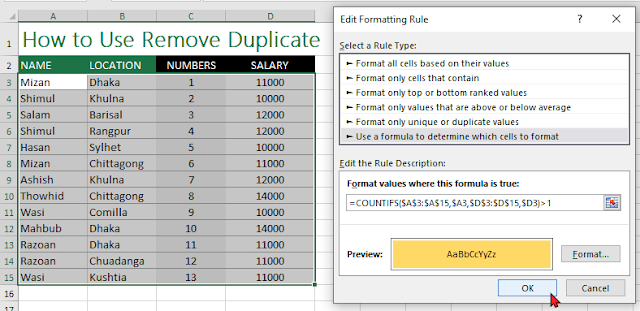
To identify duplicate records through conditional formatting, follow below steps:
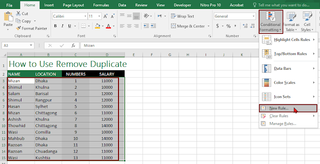
1. Select the Data Table (do not select the Header Row)
2. Click on Conditional Formatting | New Rules
3. Select Use a formula to determine which cells to format
4. Use this formula =COUNTIFS($A$3:$A$15,$A3,$D$3:$D$15,$D3)>1
5. Click on Format
6. Select a Fill Color
7. Click Ok
8. Click Ok again
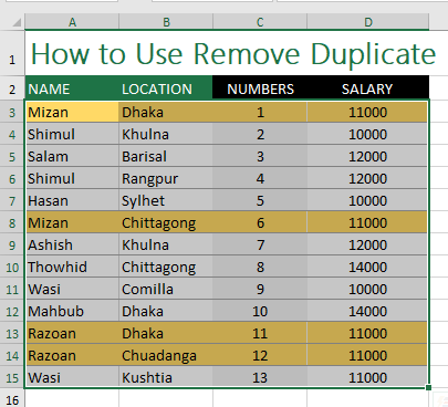
You will see Excel highlighted all the duplicate records where Name and Salary is same.
B) Through Formula:
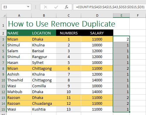
1. In E3 cell enter below formula:
=COUNTIFS($A$3:$A$15,$A3,$D$3:$D$15,$D3)
2. Copy down the formula to $D$15 cell
You will see that, The record which has Number 2, is a duplicate record.
Remove Duplicates Excel Shortcut:
The shortcut key of Remove Duplicate command is:
ALT + A + M
Excel Remove Duplicates Formula:
1. In our data table use this formula and copy down to row 15:
=COUNTIFS($A$3:$A3,$A3,$D$3:$D3,$D3)
2. In this formula the number 1 is the unique record and 2 or more than 2 numbers are duplicate.
Remove Duplicates Not Working Trouble Shooting:
A) Number Problems:
Make sure that, your number is correct. To do this, use a simple TRUE FALSE check. For example: if =D3=D5 returns FALSE, then check that number may contains decimal like 1.0000000001 and that is why =1=1.0000000001 returns FALSE. So, check properly.
B) Text Problems:
Make sure that, your number is not TEXT. If your number contains an extra space or non printed character, then =64="64 " will return FALSE. Because Non Printed Characters or Extra Space converts your Number to a TEXT.
Video Tutorial:






Comments